类神经网络训练不起来怎么办？

概念

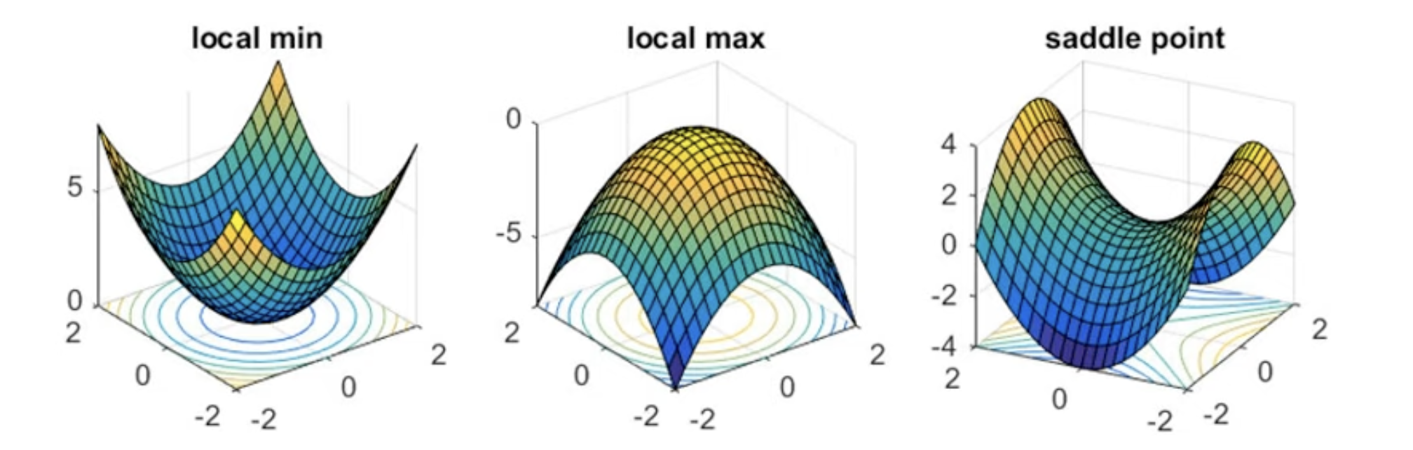
Critical Points

• Local minima
• Local maxima
• Saddle point (马鞍)

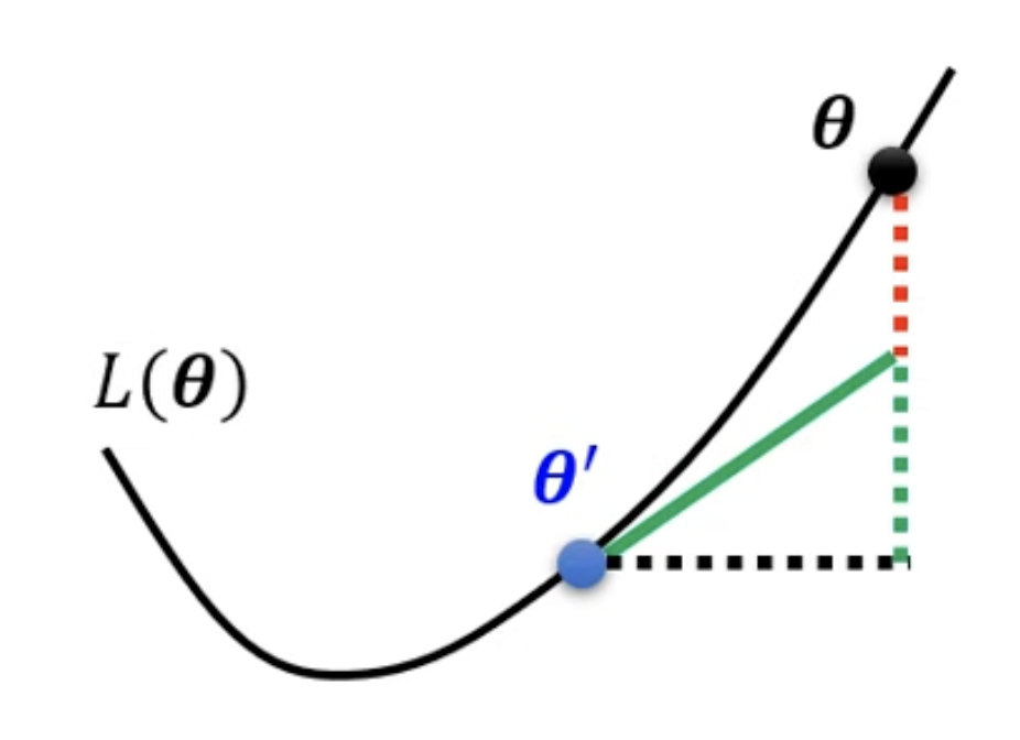
Tayler Series Approximation

The loss function $( L(\theta) )$ around $( \theta = \theta' )$ can be approximated as:

$$[ L(\theta) \approx L(\theta') + (\theta - \theta')^T g + \frac{1}{2} (\theta - \theta')^T H(\theta - \theta') ]$$

Gradient ( g ) is a vector:

$$[ g = \nabla L(\theta') \quad \text{where} \quad g_i = \frac{\partial L(\theta')}{\partial \theta_i} ]$$

Hessian ( H ) is a matrix:

$$[ H\_{ij} = \frac{\partial^2}{\partial \theta_i \partial \theta_j} L(\theta') ]$$

Optimizers

Adam: RMSProp + Momentum

• [[blog/2025-06-30-blog-082-machine-learning-training-guide/index#训练技术#Adaptive Learning Rate 技术#RMSProp]]
• [[blog/2025-06-30-blog-082-machine-learning-training-guide/index#训练技术#Momentum 技术]]

Summary of optimization

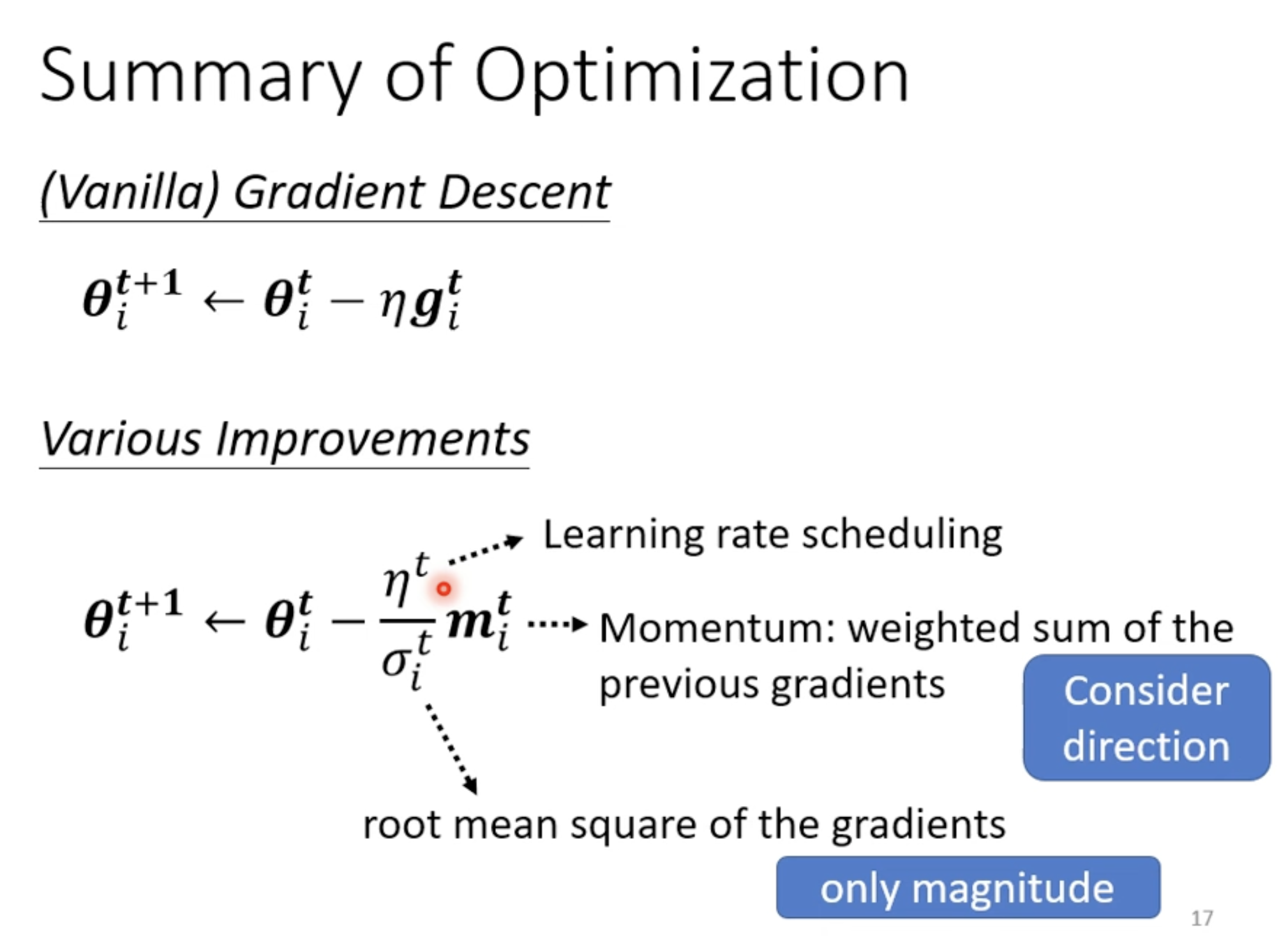
• 算不同的 momentum
• 算不同的 $\sigma$
• 算不通的 $\eta$

讨论

No local minima

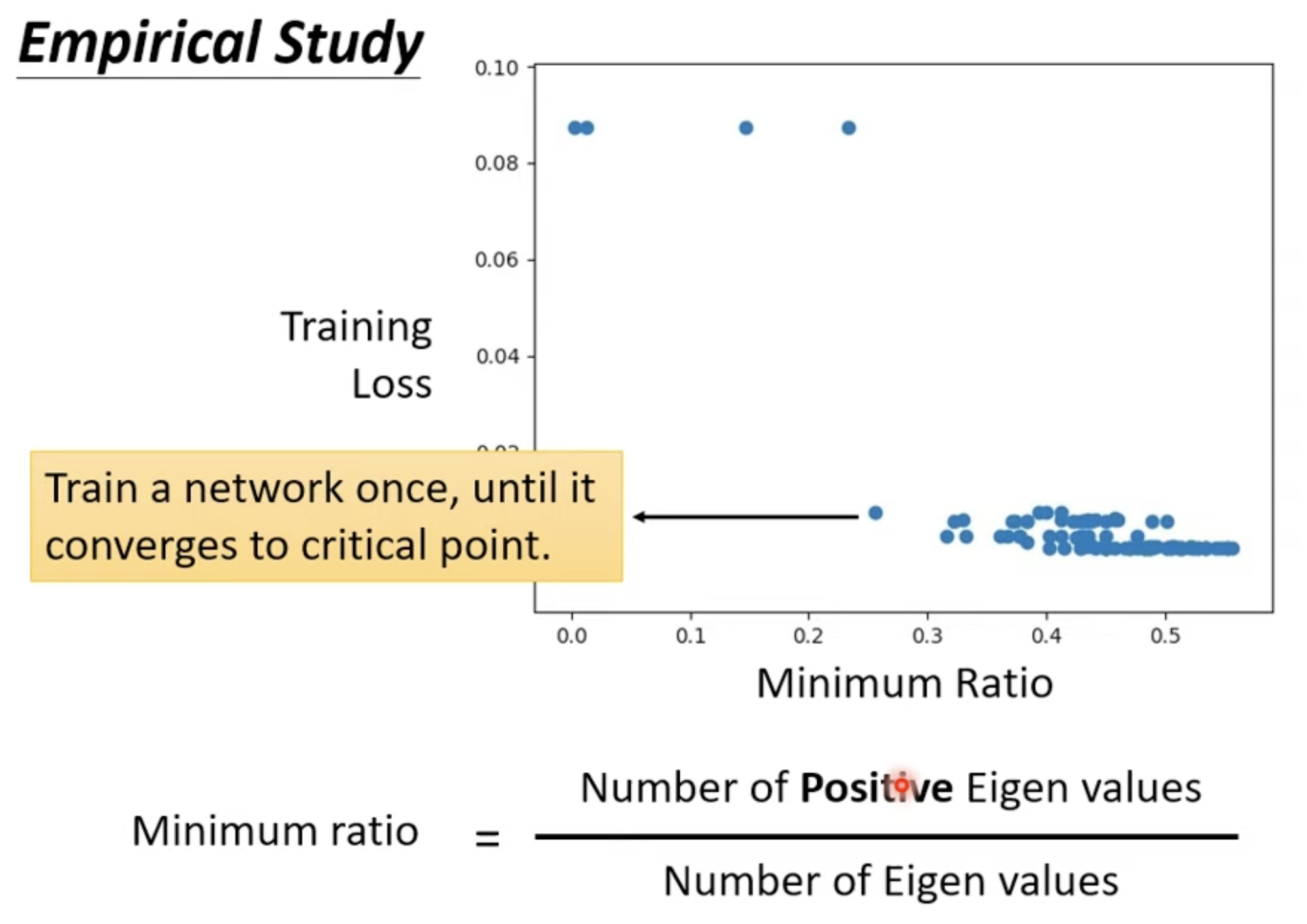
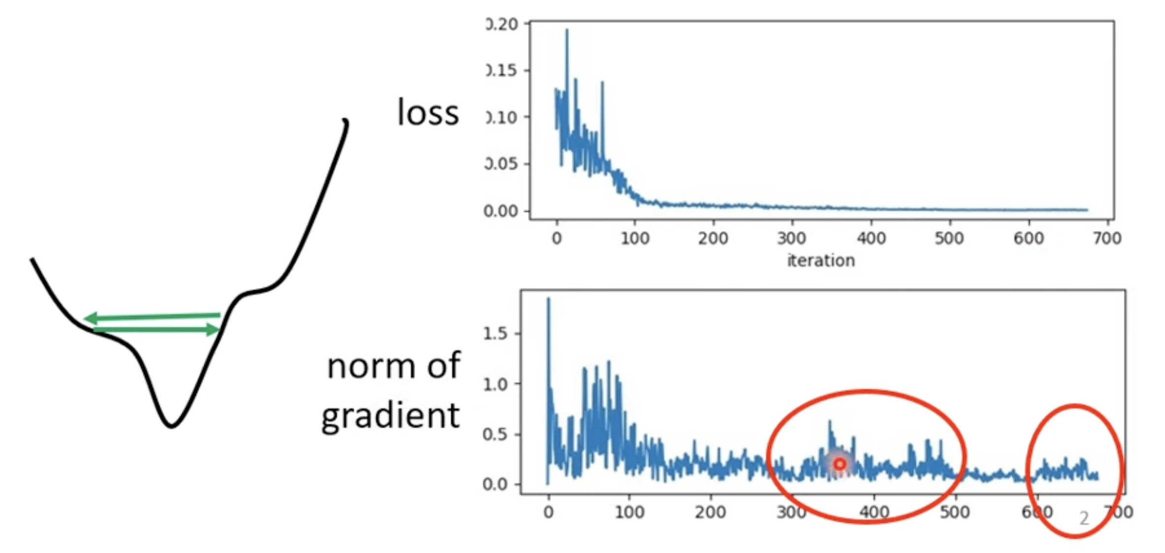
根据研究，我们其实很难找到 local minima, 因为 minimum ration 和图上的研究，我们获得最好的 Loss 的时候， Minimum Ration 大概就在 0.6 左右，这意味着我们其实还可以继续往 loss 更低的方向继续走；但是为什么训练可以停下来了呢，一个是成本问题，继续往下训练带来的成本增加和获得效果不成正比，二是你可能卡在了一个 saddle point.

Training stuck != Small Gradient

• [[blog/2025-06-30-blog-082-machine-learning-training-guide/index#训练技术#Adaptive Learning Rate 技术]]

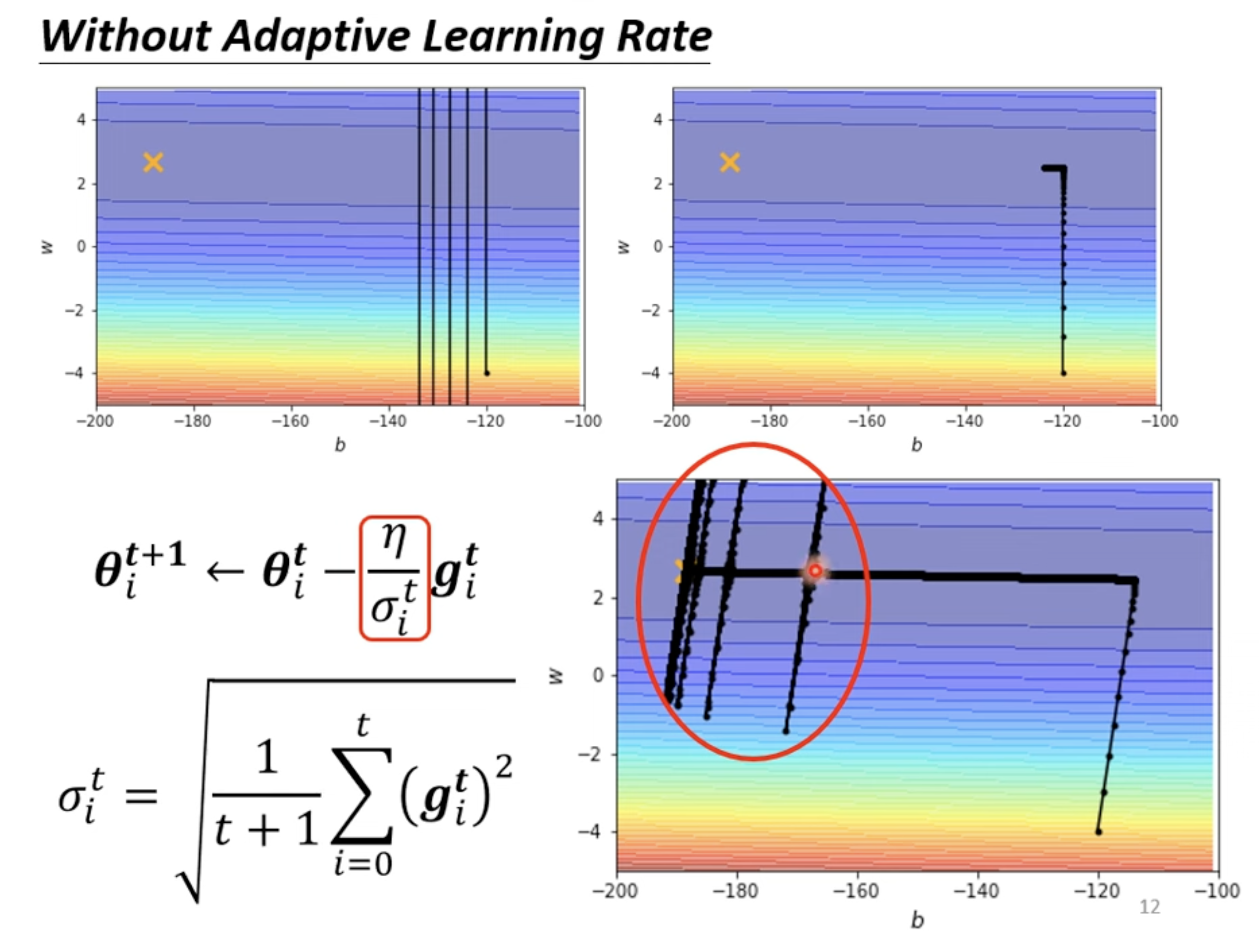
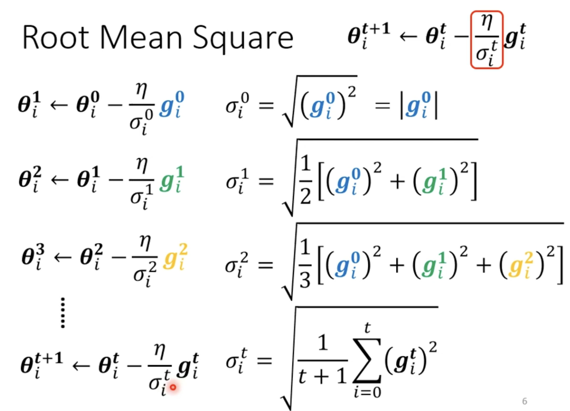
With Root Mean Square

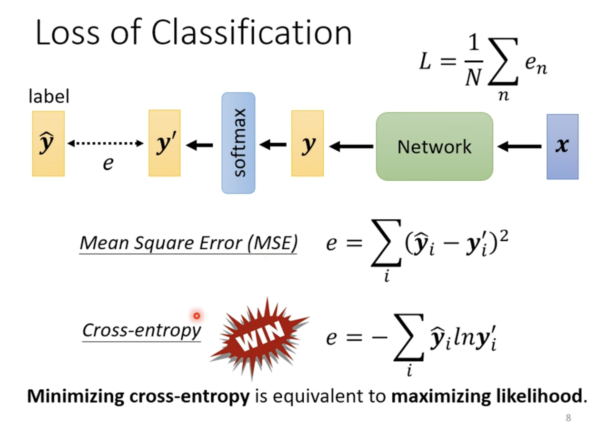
分类问题

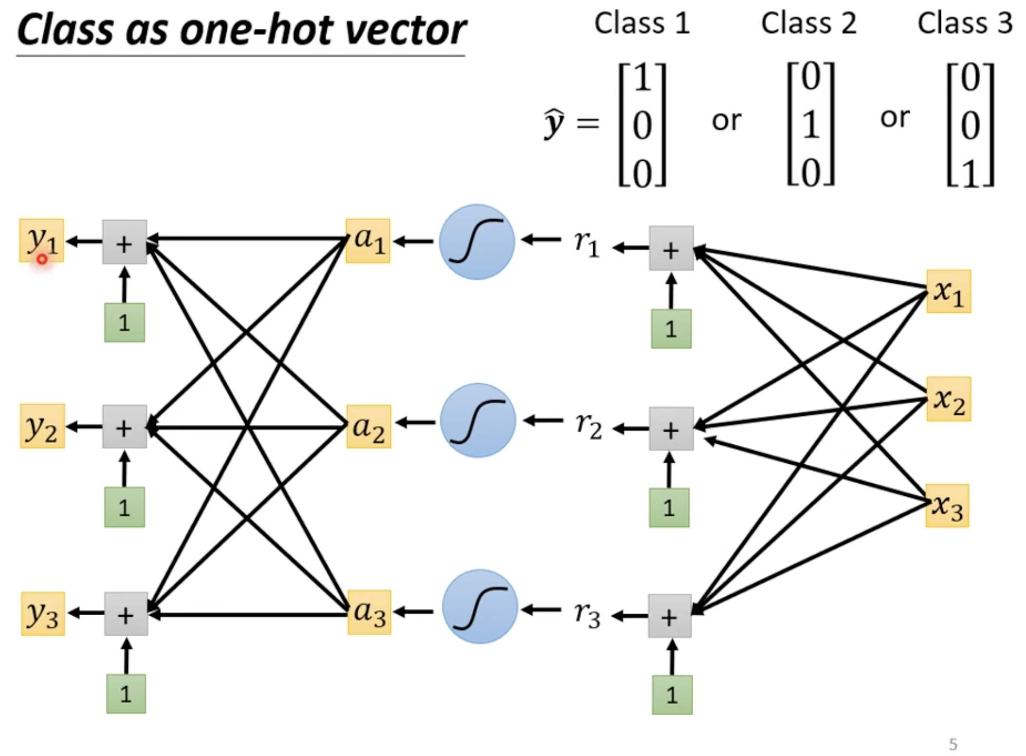
Regression vs Classification

• Regression 中 y 是一个数值，Classification 中 y 是一个向量
• softmax 将所有数值映射到 [0, 1] 的区间中，以利于后续做分类 (简单解释)

Softmax 运作

$$[ y_i' = \frac{\exp(y_i)}{\sum_{j} \exp(y_j)} ]$$

• $1 > y_i' > 0$
• $\sum_{j} \exp(y_j')$ = 1

Loss of Classification

训练技术

Batch 技术: Small Batch vs. Large Batch

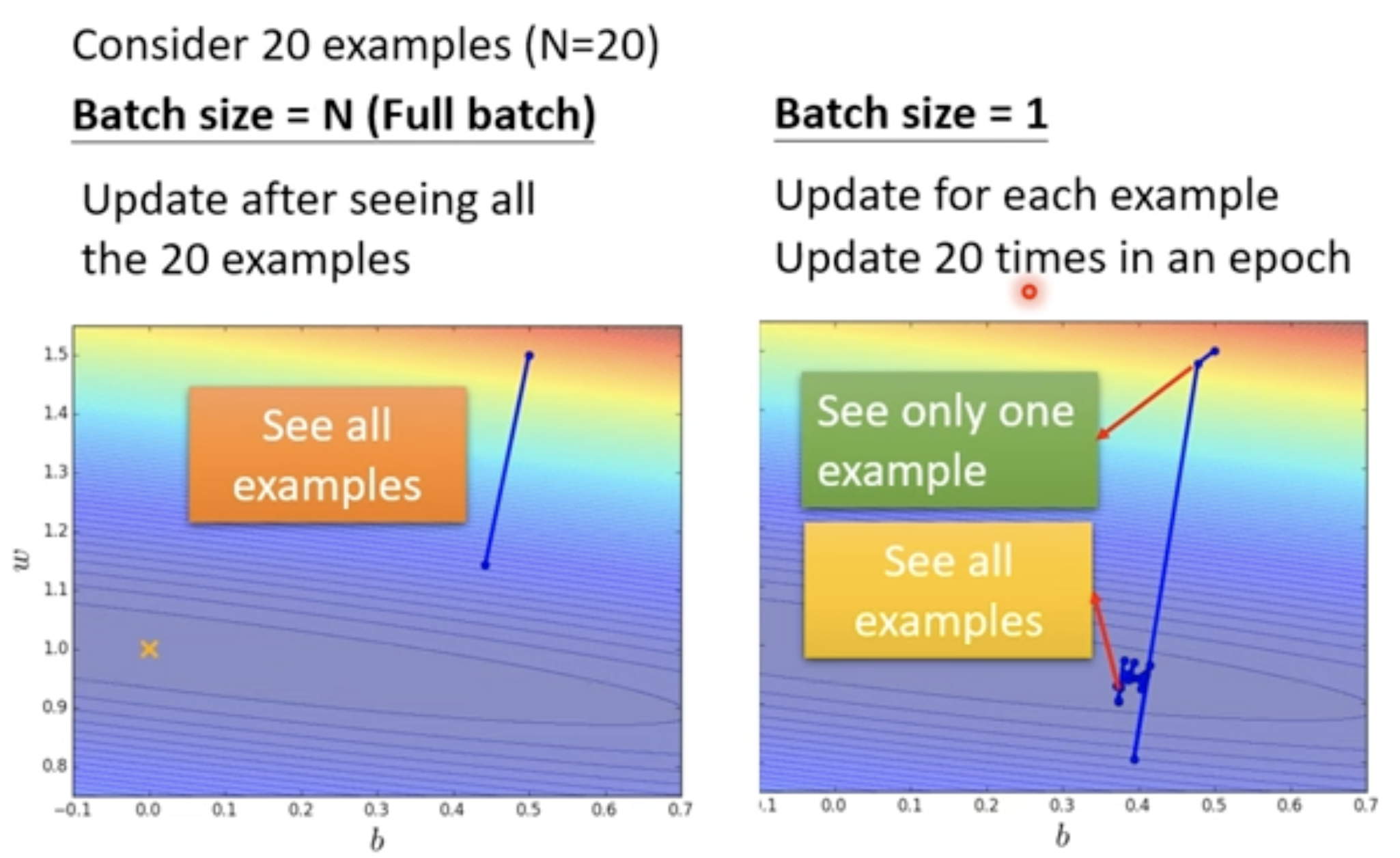
Metric	Small Batch	Large Batch
Speed for one update (no parallel)	Faster	Slower
Speed for one update (with parallel)	Same	Same (not too large)
Time for one epoch	Slower	Faster ✅
Gradient	Noisy	Stable
Optimization	Better ✅	Worse
Generalization	Better ✅	Worse

Momentum 技术

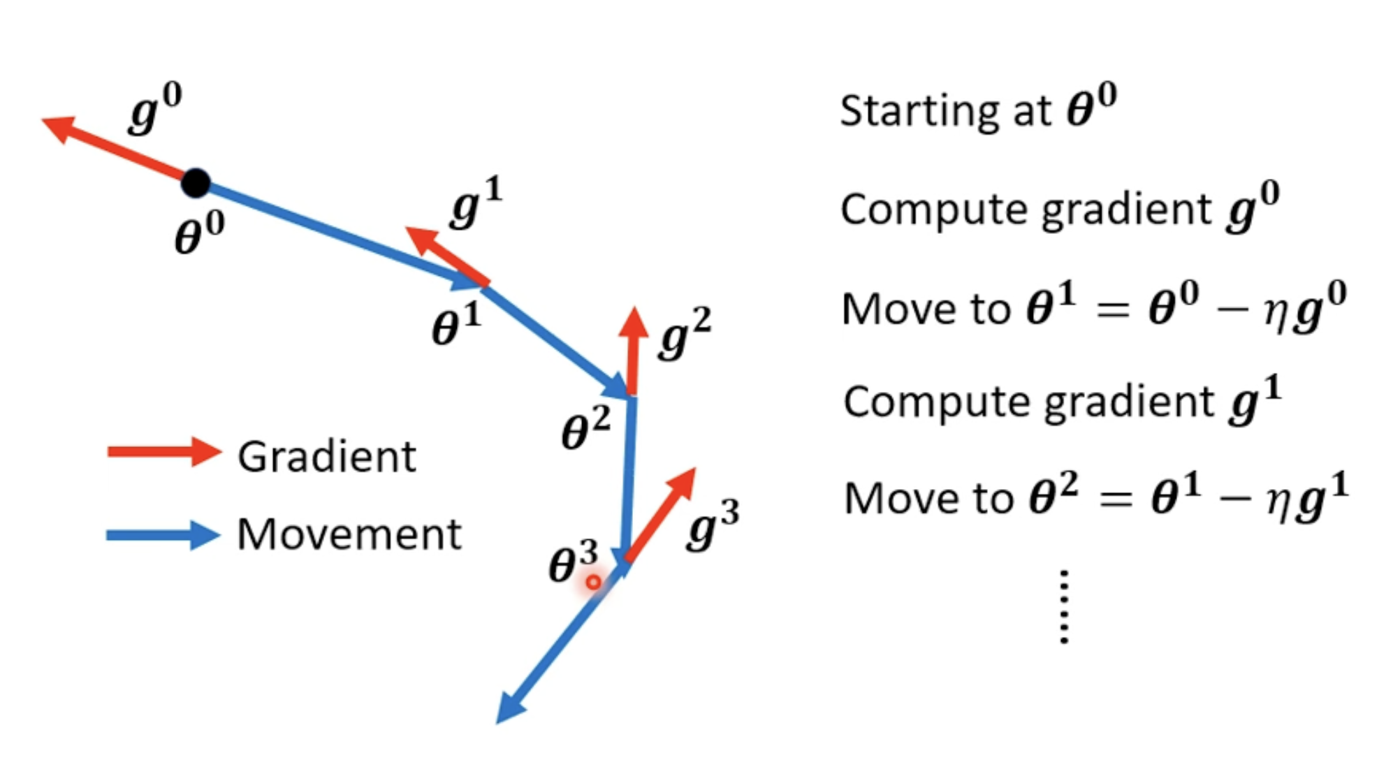
(Vanilla) Gradient Descent

Gradient Descent + Momentum

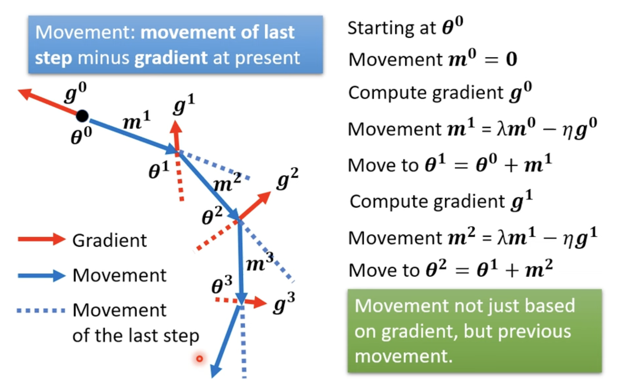
$m^i$ is the weighted sum of all the previous gradient: $g^0, g^1, ..., g^(i-1)$:

$$m^0 = 0$$ $$m^1 = -\eta g^0$$ $$m^2 = -\lambda \eta g^0 - \eta g^1$$ $$...$$

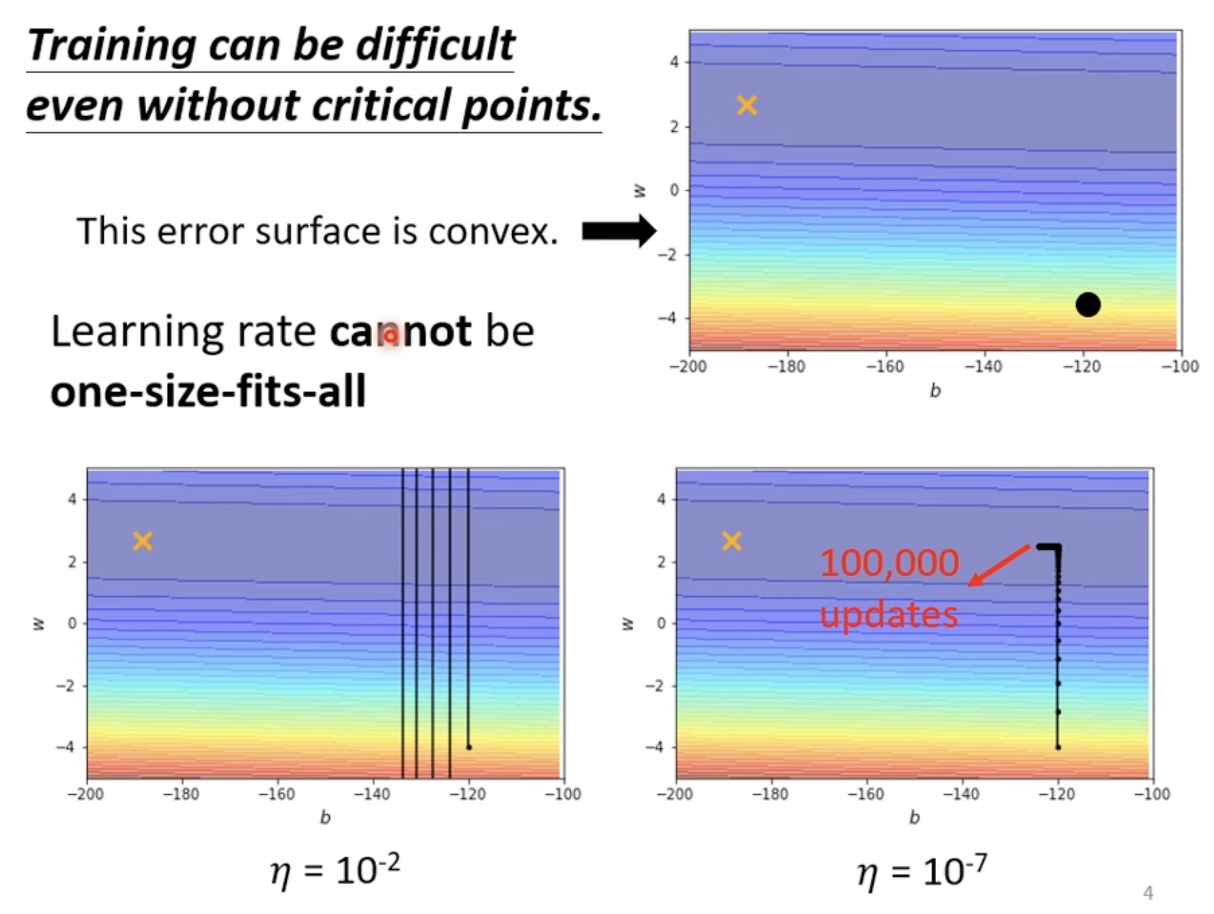
Adaptive Learning Rate 技术

$$[ \theta_i^{t+1} \leftarrow \theta_i^t - \eta g_i^t ]$$ $$[ g_i^t = \left.\frac{\partial L}{\partial \theta_i}\right|_{\theta=\theta^t} ]$$ $$[ \theta_i^{t+1} \leftarrow \theta_i^t - \frac{\eta}{\sigma_i^t} g_i^t ]$$

• $\sigma_i^t$: Parameter dependant

Root Mean Square

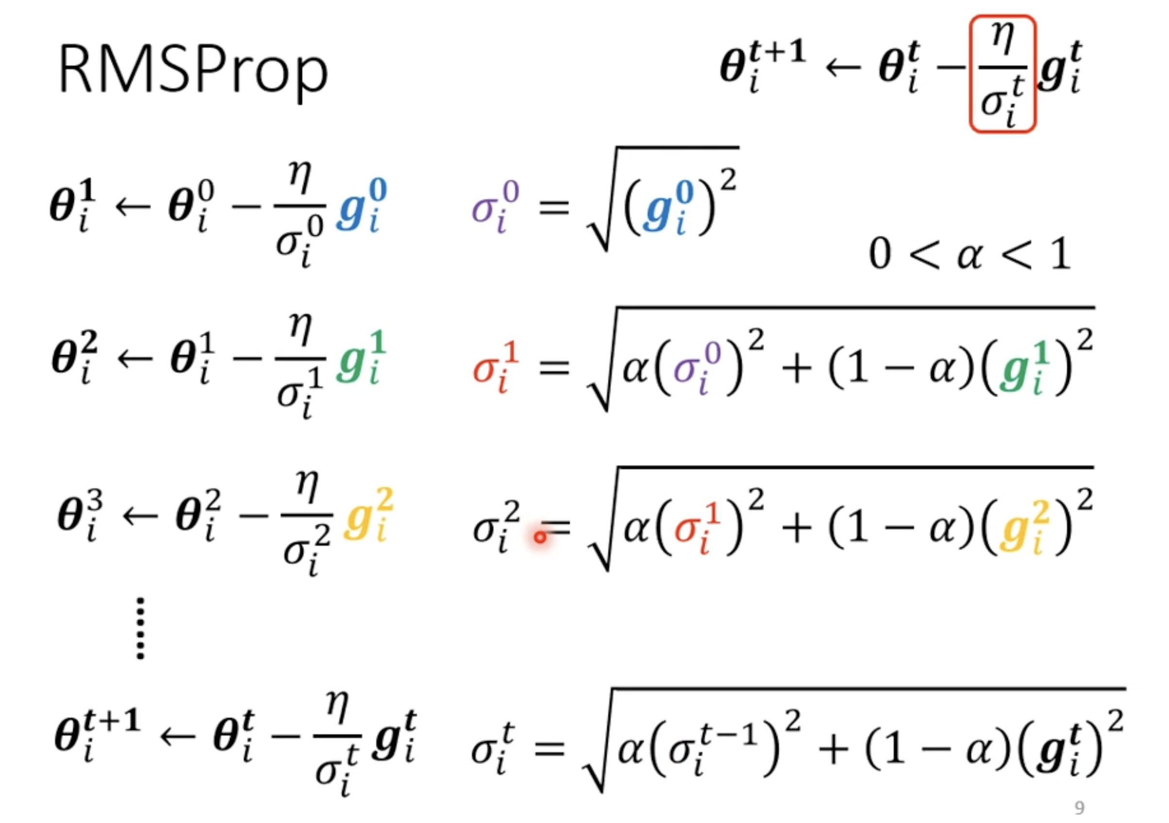
RMSProp

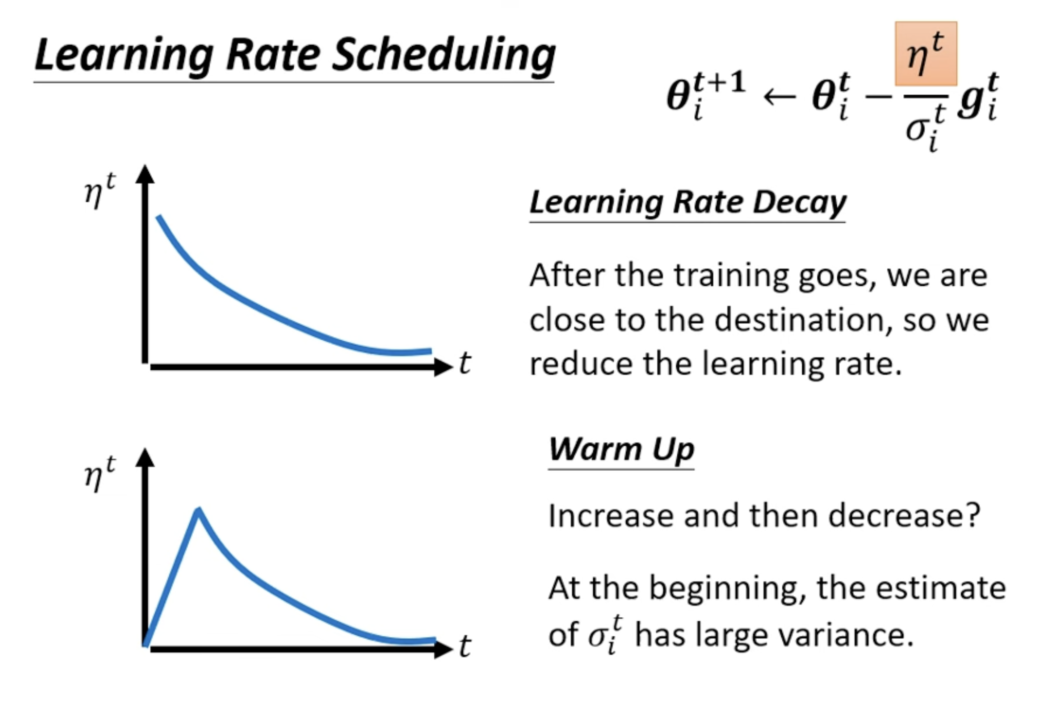
Learning Rate Scheduling

Learning Rate Decay: reduce learning rate by time.

Batch Normalization

Change landscape

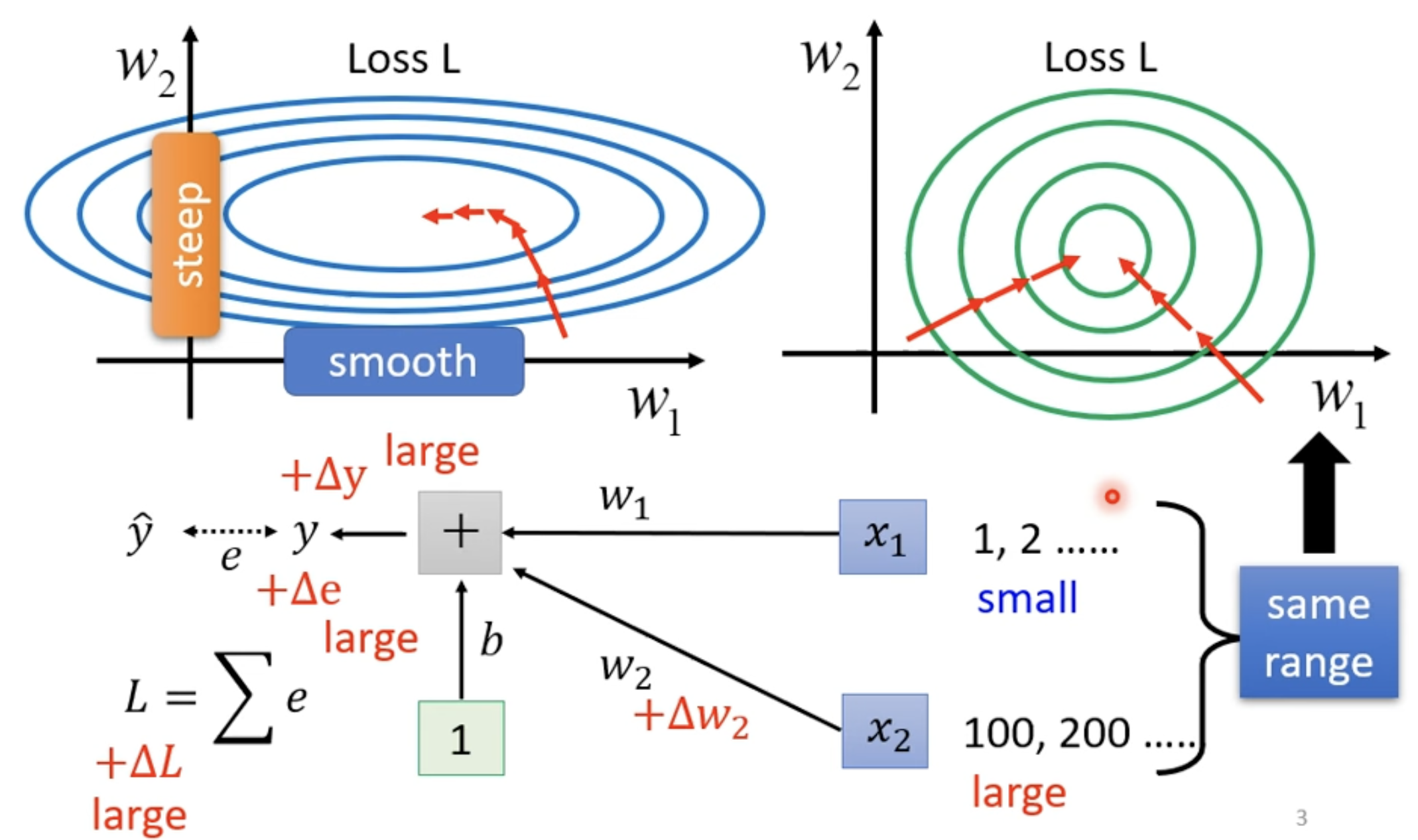
• 由于 $x_1$ 中 数值比较小，Loss 改变也会比较小；反之 $x_2$ 数值比较大，Loss 改变会比较大
• 改 Error surface，把"山"铲平

Feature Normalization

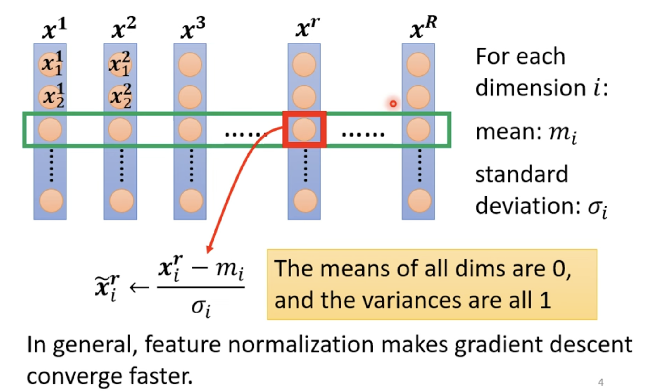
The variances are all 1 意味着 $\sigma=1$，也说明 68.2% 的数值都会在 [0, 1] 的区间，数值的分布变得更加均匀。。

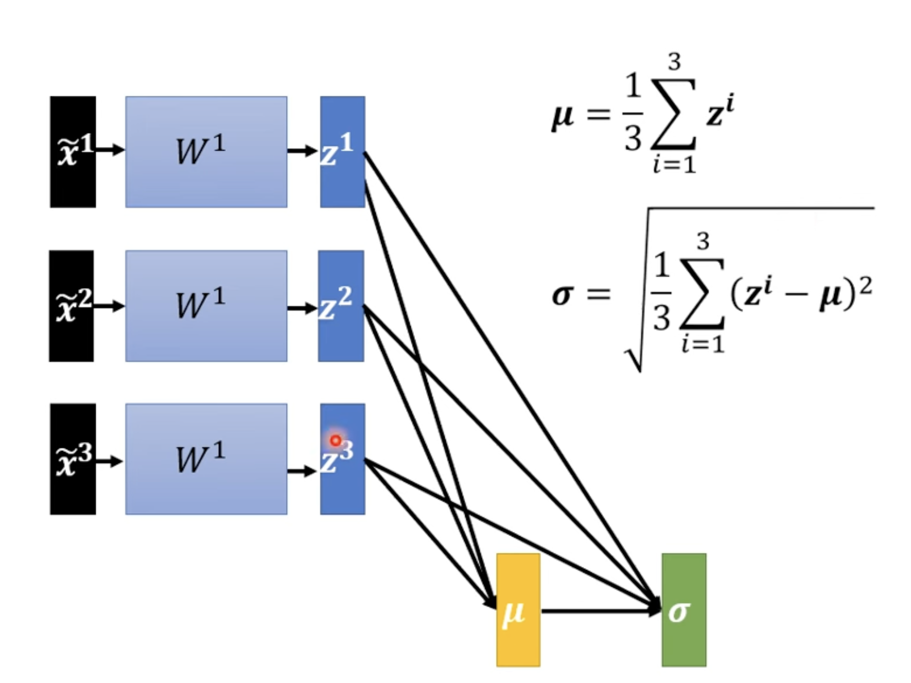
Considering Deep Learning

同样可以考虑对所有 其他位置，其他输入，其他输出做相关的 Normalization。

$$\widetilde{z}^i = \frac{\widetilde{z}^i - \mu}{\sigma}$$

做完 Feature normalization 之后，$\widetilde{z}_1$ 改变后，$\mu$ 和 $\sigma$ 改变，这会导致 $\widetilde{z}_2$ 和 $\widetilde{z}_3$, 以及之后的 $a^1$, $a^2$, $a^3$ 改变。也就是说通过 normalization 计算后获得了大的 network 里面的一部分，这对计算资源有很大的要求。

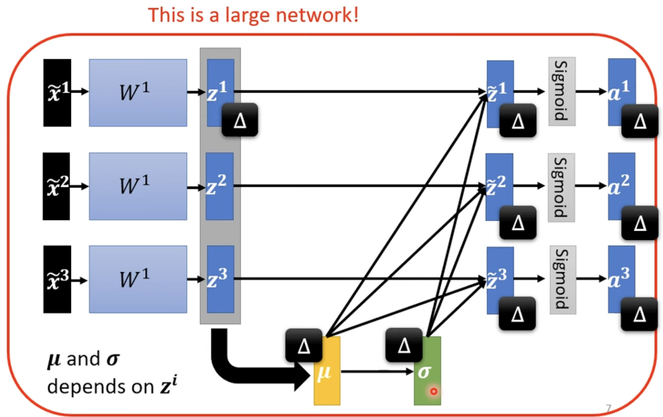
所以为了解决问题，我们将数据分为不同的 batch，算一个 batch 的话对计算资源我们是能够满足的 --> Batch Normalization(适用于 Batch Size 比较大的情况)。

Batch Normalization

Traning phase

$$\hat{Z}^i = \gamma \odot \tilde{Z}^i + \beta$$

• 当 $\hat{Z}^i$ 结果平均是 0 的话，会对结果有什么影响，为了避免这个情况，增加 $\gamma$, $\beta$;
• 所以初期的时候， $\gamma$ 全部是 1 的向量， $\beta$ 全部是 0 的向量；训练到后期在加入$\gamma$, $\beta$ 获得其他结果;
• 总的来说，加入 $\gamma$, $\beta$ 往往对训练是有好处的。

Testing phase

• 术语: inference --> testing
• Testing 没法获得一个 batch size 资料后做计算，你需要单笔进来就计算，所以 $\mu$ 和 $\sigma$ 没法获得。
• PyTorch 的解法是: Computing the moving average of $\bar{\mu}$ and $\bar{\sigma}$ of the batches during training.

• p: 0.1 (default)

Other Normalization Techniques in Deep Learning

• Batch Renormalization
  arXiv:1702.03275
  Extension of batch normalization for small batch sizes

• Layer Normalization
  arXiv:1607.06450
  Normalizes activations across features for RNNs/Transformers

• Instance Normalization
  arXiv:1607.08022
  Used in style transfer, normalizes each sample individually

• Group Normalization
  arXiv:1803.08494
  Divides channels into groups, independent of batch size

• Weight Normalization
  arXiv:1602.07868
  Rewrites weight vectors in terms of length and direction

• Spectral Normalization
  arXiv:1705.10941
  Controls Lipschitz constant in GANs via weight matrix scaling